Who applies the laws of large numbers in life. The law of large numbers in the Chebyshev form. Law of Large Numbers in Chebyshev Form: Complement

Function F(x) sometimes called integral function distribution or integral distribution law.

Distribution function properties:

1. The distribution function of a random variable is a non-negative function enclosed between zero and one:

0 ≤ F(x) ≤ 1.

2. The distribution function of a random variable is a non-decreasing function on the whole number axis.

3. At minus infinity, the distribution function is equal to zero, at plus infinity it is equal to one, i.e.: F(-∞)= , F(+∞)= .

4. The probability of a random variable falling into the interval [x1,x2) (including x1) is equal to the increment of its distribution function on this interval, i.e. P(x 1 ≤ X< х 2) = F(x 2) - F(x 1).

Markov and Chebyshev inequality

Markov inequality

Theorem: If a random variable X takes only non-negative values ​​and has a mathematical expectation, then for any positive number A the equality is true: P(x>A) ≤ .

Since the events X > A and X ≤ A are opposite, replacing P(X > A) we express 1 - P (X ≤ A), we arrive at another form of Markov's inequality: P(X ≥ A) ≥1 - .

Markov's inequality k is applicable to any non-negative random variables.

Chebyshev's inequality

Theorem: For any random variable with mathematical expectation and variance, Chebyshev's inequality is true:

P (|X - a| > ε) ≤ D(X) / ε 2 or P (|X - a| ≤ ε) ≥ 1 - DX / ε 2, where a \u003d M (X), ε>0.

Law big numbers"in the form" of Chebyshev's theorem.

Chebyshev's theorem: If the variances n independent random variables X1, X2,…. X n are limited by the same constant, then with an unlimited increase in the number n the arithmetic mean of random variables converges in probability to their arithmetic mean mathematical expectations a 1, a 2 ...., a n , i.e. .

The meaning of the law of large numbers is that the average values ​​of random variables tend to their mathematical expectation when n→ ∞ in probability. The deviation of the average values ​​from the mathematical expectation becomes arbitrarily small with a probability close to one if n is large enough. In other words, the probability of any deviation of the means from a arbitrarily small with growth n.

30. Bernoulli's theorem.

Bernoulli's theorem: Event frequency in n repeated independent trials, in each of which it can occur with the same probability p, with an unlimited increase in the number n converge in probability to the probability p of this event in a separate trial: \

Bernoulli's theorem is a consequence of Chebyshev's theorem, because the frequency of an event can be represented as the arithmetic mean of n independent alternative random variables that have the same distribution law.

18. Mathematical expectation of a discrete and continuous random variable and their properties.

mathematical expectation is the sum of the products of all its values ​​and their corresponding probabilities

For a discrete random variable:

For a continuous random variable:

Properties of mathematical expectation:

1. The mathematical expectation of a constant value is equal to the constant itself: M(S)=S

2. The constant factor can be taken out of the expectation sign, i.e. M(kX)=kM(X).

3. The mathematical expectation of the algebraic sum of a finite number of random variables is equal to the same sum of their mathematical expectations, i.e. M(X±Y)=M(X)±M(Y).

4. The mathematical expectation of the product of a finite number of independent random variables is equal to the product of their mathematical expectations: M(XY)=M(X)*M(Y).

5. If all values ​​of a random variable are increased (decreased) by a constant C, then the mathematical expectation of this random variable will increase (decrease) by the same constant C: M(X±C)=M(X)±C.

6. The mathematical expectation of the deviation of a random variable from its mathematical expectation is zero: M=0.

The words about large numbers refer to the number of tests - a large number of values ​​​​of a random variable or the cumulative action of a large number of random variables are considered. The essence of this law is as follows: although it is impossible to predict what value a single random variable will take in a single experiment, however, the total result of the action of a large number of independent random variables loses its random character and can be predicted almost reliably (i.e. with high probability). For example, it is impossible to predict which side a coin will fall on. However, if you toss 2 tons of coins, then with great certainty it can be argued that the weight of the coins that fell with the coat of arms up is 1 ton.

First of all, the so-called Chebyshev inequality refers to the law of large numbers, which estimates in a separate test the probability of a random variable accepting a value that deviates from the average value by no more than a given value.

Chebyshev's inequality. Let X is an arbitrary random variable, a=M(X) , a D(X) is its dispersion. Then

Example. The nominal (i.e. required) value of the diameter of the sleeve machined on the machine is 5mm, and the variance is no more 0.01 (this is the accuracy tolerance of the machine). Estimate the probability that in the manufacture of one bushing, the deviation of its diameter from the nominal will be less than 0.5mm .

Solution. Let r.v. X- the diameter of the manufactured bushing. By condition, its mathematical expectation is equal to the nominal diameter (if there is no systematic failure in setting up the machine): a=M(X)=5 , and the variance D(X)≤0.01. Applying the Chebyshev inequality for ε = 0.5, we get:

Thus, the probability of such a deviation is quite high, and therefore we can conclude that in the case of a single production of a part, it is almost certain that the deviation of the diameter from the nominal will not exceed 0.5mm .

Basically, the standard deviation σ characterizes average deviation of a random variable from its center (i.e. from its mathematical expectation). Because it average deviation, then large deviations (emphasis on o) are possible during testing. How large deviations are practically possible? When studying normally distributed random variables, we derived the “three sigma” rule: a normally distributed random variable X in a single test practically does not deviate from its average further than 3σ, where σ= σ(X) is the standard deviation of r.v. X. We deduced such a rule from the fact that we obtained the inequality

.

Let us now estimate the probability for arbitrary random variable X accept a value that differs from the mean by no more than three times the standard deviation. Applying the Chebyshev inequality for ε = 3σ and given that D(X)=σ 2 , we get:

.

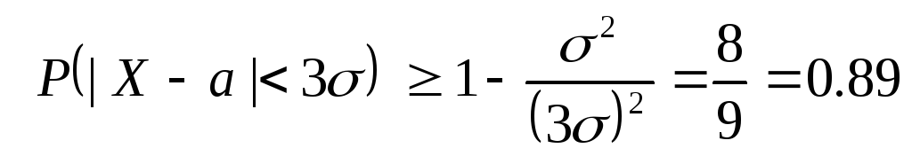In this way, in general we can estimate the probability of a random variable deviating from its mean by no more than three standard deviations by the number 0.89 , while for a normal distribution it can be guaranteed with probability 0.997 .

Chebyshev's inequality can be generalized to a system of independent identically distributed random variables.

Generalized Chebyshev's inequality. If independent random variables X 1 , X 2 , … , X n M(X i )= a and dispersions D(X i )= D, then

At n=1 this inequality goes over into the Chebyshev inequality formulated above.

The Chebyshev inequality, having independent significance for solving the corresponding problems, is used to prove the so-called Chebyshev theorem. We first describe the essence of this theorem and then give its formal formulation.

Let X 1 , X 2 , … , X n– a large number of independent random variables with mathematical expectations M(X 1 )=a 1 , … , M(X n )=a n. Although each of them, as a result of the experiment, can take a value far from its average (i.e., mathematical expectation), however, a random variable
, equal to their arithmetic mean, with a high probability will take a value close to a fixed number
(this is the average of all mathematical expectations). This means the following. Let, as a result of the test, independent random variables X 1 , X 2 , … , X n(there are a lot of them!) have taken the values ​​accordingly X 1 , X 2 , … , X n respectively. Then if these values ​​themselves may turn out to be far from the average values ​​of the corresponding random variables, their average value
is likely to be close to
. Thus, the arithmetic mean of a large number of random variables already loses its random character and can be predicted with great accuracy. This can be explained by the fact that random deviations of the values X i from a i can be of different signs, and therefore in total these deviations are compensated with a high probability.

Terema Chebysheva (law of large numbers in the form of Chebyshev). Let X 1 , X 2 , … , X n … is a sequence of pairwise independent random variables whose variances are limited to the same number. Then, no matter how small the number ε we take, the probability of inequality

will be arbitrarily close to unity if the number n random variables to take large enough. Formally, this means that under the conditions of the theorem

This type of convergence is called convergence in probability and is denoted by:

Thus, Chebyshev's theorem says that if there are a sufficiently large number of independent random variables, then their arithmetic mean in a single test will almost certainly take a value close to the mean of their mathematical expectations.

Most often, the Chebyshev theorem is applied in a situation where random variables X 1 , X 2 , … , X n … have the same distribution (i.e. the same distribution law or the same probability density). In fact, this is just a large number of instances of the same random variable.

Consequence(of the generalized Chebyshev inequality). If independent random variables X 1 , X 2 , … , X n … have the same distribution with mathematical expectations M(X i )= a and dispersions D(X i )= D, then

, i.e.
.

The proof follows from the generalized Chebyshev inequality by passing to the limit as n→∞ .

We note once again that the equalities written above do not guarantee that the value of the quantity
tends to a at n→∞. This value is still a random variable, and its individual values ​​can be quite far from a. But the probability of such (far from a) values ​​with increasing n tends to 0.

Comment. The conclusion of the corollary is obviously also valid in the more general case when the independent random variables X 1 , X 2 , … , X n … have a different distribution, but the same mathematical expectations (equal a) and the variances limited in the aggregate. This makes it possible to predict the accuracy of measuring a certain quantity, even if these measurements are made by different instruments.

Let us consider in more detail the application of this corollary to the measurement of quantities. Let's use some device n measurements of the same quantity, the true value of which is a and we don't know. The results of such measurements X 1 , X 2 , … , X n may differ significantly from each other (and from the true value a) due to various random factors (pressure drops, temperatures, random vibration, etc.). Consider the r.v. X- instrument reading for a single measurement of a quantity, as well as a set of r.v. X 1 , X 2 , … , X n- instrument reading at the first, second, ..., last measurement. Thus, each of the quantities X 1 , X 2 , … , X n there is just one of the instances of the r.v. X, and therefore they all have the same distribution as the r.v. X. Since the measurement results are independent of each other, the r.v. X 1 , X 2 , … , X n can be considered independent. If the device does not give a systematic error (for example, zero is not “knocked down” on the scale, the spring is not stretched, etc.), then we can assume that the mathematical expectation M(X) = a, and therefore M(X 1 ) = ... = M(X n ) = a. Thus, the conditions of the above corollary are satisfied, and therefore, as an approximate value of the quantity a we can take the "implementation" of a random variable
in our experiment (consisting of a series of n measurements), i.e.

.

At large numbers measurements, the good accuracy of the calculation according to this formula is practically reliable. This is the rationale for the practical principle that, with a large number of measurements, their arithmetic mean practically does not differ much from the true value of the measured quantity.

The “selective” method, which is widely used in mathematical statistics, is based on the law of large numbers, which allows obtaining its objective characteristics with acceptable accuracy from a relatively small sample of values ​​of a random variable. But this will be discussed in the next section.

Example. On a measuring device that does not make systematic distortions, a certain quantity is measured a once (received value X 1 ), and then another 99 times (obtained values X 2 , … , X 100 ). For the true value of measurement a first take the result of the first measurement
, and then the arithmetic mean of all measurements
. The measurement accuracy of the device is such that the standard deviation of the measurement σ is not more than 1 (because the dispersion D=σ 2 also does not exceed 1). For each of the measurement methods, estimate the probability that the measurement error does not exceed 2.

Solution. Let r.v. X- instrument reading for a single measurement. Then by condition M(X)=a. To answer the questions posed, we apply the generalized Chebyshev inequality

for ε =2 first for n=1 and then for n=100 . In the first case, we get
, and in the second. Thus, the second case practically guarantees the given measurement accuracy, while the first one leaves serious doubts in this sense.

Let us apply the above statements to the random variables that arise in the Bernoulli scheme. Let us recall the essence of this scheme. Let it be produced n independent tests, in each of which some event BUT can appear with the same probability R, a q=1–r(by meaning, this is the probability of the opposite event - not the occurrence of an event BUT) . Let's spend some number n such tests. Consider random variables: X 1 – number of occurrences of the event BUT in 1 th test, ..., X n– number of occurrences of the event BUT in n th test. All introduced r.v. can take values 0 or 1 (event BUT may appear in the test or not), and the value 1 conditionally accepted in each trial with a probability p(probability of occurrence of an event BUT in each test), and the value 0 with probability q= 1 – p. Therefore, these quantities have the same distribution laws:

Therefore, the average values ​​of these quantities and their dispersions are also the same: M(X 1 )=0 ∙ q+1 ∙ p= p, …, M(X n )= p ; D(X 1 )=(0 2 ∙ q+1 2 ∙ p)− p 2 = p∙(1− p)= p ∙ q, … , D(X n )= p ∙ q . Substituting these values ​​into the generalized Chebyshev inequality, we obtain

.

It is clear that the r.v. X=X 1 +…+Х n is the number of occurrences of the event BUT in all n trials (as they say - "the number of successes" in n tests). Let in the n test event BUT appeared in k of them. Then the previous inequality can be written as

.

But the magnitude
, equal to the ratio of the number of occurrences of the event BUT in n independent trials, to the total number of trials, previously called the relative event rate BUT in n tests. Therefore, there is an inequality

.

Passing now to the limit at n→∞, we get
, i.e.
(according to probability). This is the content of the law of large numbers in the form of Bernoulli. It follows from this that for a sufficiently large number of trials n arbitrarily small deviations of the relative frequency
events from its probability R are almost certain events, and large deviations are almost impossible. The resulting conclusion about such stability of relative frequencies (which we previously referred to as experimental fact) justifies the previously introduced statistical definition of the probability of an event as a number around which the relative frequency of an event fluctuates.

Considering that the expression p∙ q= p∙(1− p)= p− p 2 does not exceed on the change interval
(it is easy to verify this by finding the minimum of this function on this segment), from the above inequality
easy to get that

,

which is used in solving the corresponding problems (one of them will be given below).

Example. The coin was flipped 1000 times. Estimate the probability that the deviation of the relative frequency of the appearance of the coat of arms from its probability will be less than 0.1.

Solution. Applying the inequality
at p= q=1/2 , n=1000 , ε=0.1, we get .

Example. Estimate the probability that, under the conditions of the previous example, the number k of the dropped coats of arms will be in the range of 400 before 600 .

Solution. Condition 400< k<600 means that 400/1000< k/ n<600/1000 , i.e. 0.4< W n (A)<0.6 or
. As we have just seen from the previous example, the probability of such an event is at least 0.975 .

Example. To calculate the probability of some event BUT 1000 experiments were carried out, in which the event BUT appeared 300 times. Estimate the probability that the relative frequency (equal to 300/1000=0.3) is different from the true probability R no further than 0.1 .

Solution. Applying the above inequality
for n=1000, ε=0.1 , we get .

The practice of studying random phenomena shows that although the results of individual observations, even those carried out under the same conditions, can differ greatly, at the same time, the average results for a sufficiently large number of observations are stable and weakly depend on the results of individual observations.

The theoretical justification for this remarkable property of random phenomena is law of large numbers. The name "law of large numbers" combines a group of theorems that establish the stability of the average results of a large number of random phenomena and explain the reason for this stability.

The simplest form of the law of large numbers, and historically the first theorem of this section is Bernoulli's theorem stating that if the probability of an event is the same in all trials, then with an increase in the number of trials, the frequency of the event tends to the probability of the event and ceases to be random.

Poisson's theorem states that the frequency of an event in a series of independent trials tends to the arithmetic mean of its probabilities and ceases to be random.

Limit theorems of probability theory, theorems Moivre-Laplace explain the nature of the stability of the frequency of occurrence of an event. This nature consists in the fact that the limiting distribution of the number of occurrences of an event with an unlimited increase in the number of trials (if the probability of an event in all trials is the same) is normal distribution.

The central limit theorem explains the widespread use normal law distribution. The theorem states that whenever a random variable is formed as a result of adding a large number of independent random variables with finite variances, the distribution law of this random variable turns out to be practically normal by law.

The theorem below, titled " Law of Large Numbers" states that under certain, fairly general, conditions, with an increase in the number of random variables, their arithmetic mean tends to the arithmetic mean of mathematical expectations and ceases to be random.

Lyapunov's theorem explains the widespread normal law distribution and explains the mechanism of its formation. The theorem allows us to assert that whenever a random variable is formed as a result of adding a large number of independent random variables, the variances of which are small compared to the variance of the sum, the distribution law of this random variable turns out to be practically normal by law. And since random variables are always generated by an infinite number of causes, and most often none of them has a variance comparable to the variance of the random variable itself, most of the random variables encountered in practice are subject to the normal distribution law.

The qualitative and quantitative statements of the law of large numbers are based on Chebyshev's inequality. It defines the upper bound on the probability that the deviation of the value of a random variable from its mathematical expectation is greater than some given number. Remarkably, the Chebyshev inequality gives an estimate of the probability of the event for a random variable whose distribution is unknown, only its mathematical expectation and variance are known.

Chebyshev's inequality. If a random variable x has a variance, then for any e > 0 the inequality , where M x and D x - mathematical expectation and variance of the random variable x .

Bernoulli's theorem. Let m n be the number of successes in n Bernoulli trials and p be the probability of success in a single trial. Then for any e > 0 we have .

Central limit theorem. If random variables x 1 , x 2 , …, x n , … are pairwise independent, equally distributed and have finite variance, then at n ® uniformly in x (- ,)

If the phenomenon of sustainability medium takes place in reality, then mathematical model, with the help of which we study random phenomena, there must be a theorem reflecting this fact.
Under the conditions of this theorem, we introduce restrictions on random variables X 1 , X 2 , …, X n:

a) each random variable Х i has mathematical expectation

M(Х i) = a;

b) the variance of each random variable is finite, or we can say that the variances are bounded from above by the same number, for example FROM, i.e.

D(Х i) < C, i = 1, 2, …, n;

c) random variables are pairwise independent, i.e. any two X i and Xj at i¹ j independent.

Then obviously

D(X 1 + X 2 + … + X n)=D(X 1) + D(X 2) + ... + D(X n).

Let us formulate the law of large numbers in the Chebyshev form.

Chebyshev's theorem: with an unlimited increase in the number n independent tests " the arithmetic mean of the observed values ​​of a random variable converges in probability to its mathematical expectation ”, i.e. for any positive ε

R(| –a| < ε ) = 1. (4.1.1)

The meaning of the expression "arithmetic mean = converges in probability to a" is that the probability that will differ arbitrarily little from a, approaches 1 indefinitely as the number n.

Proof. For a finite number n independent tests, we apply the Chebyshev inequality for a random variable = :

R(|–M()| < ε ) ≥ 1 – . (4.1.2)

Taking into account the restrictions a - b, we calculate M( ) and D( ):

M( ) = = = = = = a;

D( ) = = = = = = .

Substituting M( ) and D( ) into inequality (4.1.2), we obtain

R(| –a| < ε )≥1 – .

If in inequality (4.1.2) we take an arbitrarily small ε >0and n® ¥, then we get

which proves the Chebyshev theorem.

An important practical conclusion follows from the considered theorem: we have the right to replace the unknown value of the mathematical expectation of a random variable by the arithmetic mean value obtained from a sufficiently large number of experiments. In this case, the more experiments to calculate, the more likely (reliable) it can be expected that the error associated with this replacement ( - a) will not exceed the given value ε .

In addition, other practical problems can be solved. For example, according to the values ​​of probability (reliability) R=R(| – a|< ε ) and the maximum allowable error ε determine the required number of experiments n; on R and P define ε; on ε and P determine the probability of an event | – a |< ε.

special case. Let at n trials observed n values ​​of a random variable x, having mathematical expectation M(X) and dispersion D(X). The obtained values ​​can be considered as random variables X 1 ,X 2 ,X 3 , ... ,X n,. It should be understood as follows: a series of P tests are carried out repeatedly, so as a result i th test, i= l, 2, 3, ..., P, in each series of tests one or another value of a random variable will appear X, not known in advance. Consequently, i-e value x i random variable obtained in i th test, changes randomly if you move from one series of tests to another. So every value x i can be considered random X i .

Assume that the tests meet the following requirements:

1. Tests are independent. This means that the results X 1 , X 2 ,
X 3 , ..., X n tests are independent random variables.

2. Tests are carried out under the same conditions - this means, from the point of view of probability theory, that each of the random variables X 1 ,X 2 ,X 3 , ... ,X n has the same distribution law as the original value X, that's why M(X i) = M(X)and D(X i) = D(X), i = 1, 2, .... P.

Considering the above conditions, we get

R(| –a| < ε )≥1 – . (4.1.3)

Example 4.1.1. X is equal to 4. How many independent experiments are required so that with a probability of at least 0.9 it can be expected that the arithmetic mean of this random variable will differ from the mathematical expectation by less than 0.5?

Solution.According to the condition of the problem ε = 0,5; R(| – a|< 0,5) ≥ 0.9. Applying formula (4.1.3) for the random variable X, we get

P(|–M(X)| < ε ) ≥ 1 – .

From the relation

1 – = 0,9

define

P= = = 160.

Answer: it is required to make 160 independent experiments.

Assuming that the arithmetic mean normally distributed, we get:

R(| – a|< ε )= 2Φ () ≥ 0,9.

From where, using the table of the Laplace function, we get ≥
≥ 1.645, or ≥ 6.58 i.e. n ≥49.

Example 4.1.2. Variance of a random variable X is equal to D( X) = 5. 100 independent experiments were carried out, according to which . Instead of the unknown value of the mathematical expectation a accepted . Determine the maximum amount of error allowed in this case with a probability of at least 0.8.

Solution. According to the task n= 100, R(| –a|< ε ) ≥0.8. We apply the formula (4.1.3)

R(| –a|< ε ) ≥1 – .

From the relation

1 – = 0,8

define ε :

ε 2 = = = 0,25.

Consequently, ε = 0,5.

Answer: maximum error value ε = 0,5.

4.2. Law of large numbers in Bernoulli form

Although the concept of probability is the basis of any statistical inference, we can only in a few cases determine the probability of an event directly. Sometimes this probability can be established from considerations of symmetry, equal opportunity, etc., but there is no universal method that would allow one to indicate its probability for an arbitrary event. Bernoulli's theorem makes it possible to approximate the probability if for the event of interest to us BUT repeated independent tests can be carried out. Let produced P independent tests, in each of which the probability of occurrence of some event BUT constant and equal R.

Bernoulli's theorem. With an unlimited increase in the number of independent trials P relative frequency of occurrence of an event BUT converges in probability to probability p occurrence of an event BUT,t. e.

P(½ - p½≤ ε) = 1, (4.2.1)

where ε is an arbitrarily small positive number.

For the final n provided that , Chebyshev's inequality for a random variable will have the form:

P(| –p|< ε ) ≥ 1 – .(4.2.2)

Proof. We apply the Chebyshev theorem. Let X i– number of occurrences of the event BUT in i th test, i= 1, 2, . . . , n. Each of the quantities X i can only take two values:

X i= 1 (event BUT happened) with a probability p,

X i= 0 (event BUT did not occur) with a probability q= 1–p.

Let Y n= . Sum X 1 + X 2 + … + X n is equal to the number m event occurrences BUT in n tests (0 m n), which means Y n= – relative frequency of occurrence of the event BUT in n tests. Mathematical expectation and variance X i are equal respectively:

M( ) = 1∙p + 0∙q = p,

Example 4.2.1. In order to determine the percentage of defective products, 1000 units were tested according to the return sampling scheme. What is the probability that the absolute value of the reject rate determined by this sample will differ from the reject rate for the entire batch by no more than 0.01, if it is known that, on average, there are 500 defective items for every 10,000 items?

Solution. According to the condition of the problem, the number of independent trials n= 1000;

p= = 0,05; q= 1 – p= 0,95; ε = 0,01.

Applying formula (4.2.2), we obtain

P(| –p|< 0,01) ≥ 1 – = 1 – = 0,527.

Answer: with a probability of at least 0.527, it can be expected that the sample fraction of defects (the relative frequency of occurrence of defects) will differ from the share of defects in all products (from the probability of defects) by no more than 0.01.

Example 4.2.2. When stamping parts, the probability of marriage is 0.05. How many parts must be checked so that with a probability of at least 0.95 it can be expected that the relative frequency of defective products will differ from the probability of defects by less than 0.01?

Solution. According to the task R= 0,05; q= 0,95; ε = 0,01;

P(| – p|<0,01) ≥ 0,95.

From equality 1 – = 0.95 find n:

n= = =9500.

Answer: 9500 items need to be checked.

Comment. Estimates of the required number of observations obtained by applying Bernoulli's (or Chebyshev's) theorem are greatly exaggerated. There are more precise estimates proposed by Bernstein and Khinchin, but requiring a more complex mathematical apparatus. To avoid exaggeration of estimates, the Laplace formula is sometimes used

P(| – p|< ε ) ≈ 2Φ .

The disadvantage of this formula is the lack of an estimate of the allowable error.

The phenomenon of stabilization of the frequencies of occurrence of random events, discovered on a large and varied material, at first did not have any justification and was perceived as a purely empirical fact. The first theoretical result in this area was the famous Bernoulli theorem published in 1713, which laid the foundation for the laws of large numbers.

Bernoulli's theorem in its content is a limit theorem, i.e., a statement of asymptotic meaning, saying what will happen to the probabilistic parameters with a large number of observations. The progenitor of all modern numerous statements of this type is precisely Bernoulli's theorem.

Today it seems that the mathematical law of large numbers is a reflection of some common property of many real processes.

Having a desire to give the law of large numbers as much coverage as possible, corresponding to the far from exhausted potential possibilities of applying this law, one of the greatest mathematicians of our century A. N. Kolmogorov formulated its essence as follows: the law of large numbers is “a general principle by virtue of which the action of a large number of random factors leads to a result almost independent of chance.

Thus, the law of large numbers has, as it were, two interpretations. One is mathematical, associated with specific mathematical models, formulations, theories, and the second is more general, going beyond this framework. The second interpretation is connected with the phenomenon of formation, which is often noted in practice, in varying degrees of directed action against the background of a large number of hidden or visible acting factors that do not have such continuity outwardly. Examples related to the second interpretation are pricing in the free market, the formation of public opinion on a particular issue.

Having noted this general interpretation of the law of large numbers, let us turn to the specific mathematical formulations of this law.

As we said above, the first and fundamentally most important for the theory of probability is Bernoulli's theorem. The content of this mathematical fact, which reflects one of the most important regularities of the surrounding world, is reduced to the following.

Consider a sequence of unrelated (i.e., independent) tests, the conditions for which are reproduced invariably from test to test. The result of each test is the appearance or non-appearance of the event of interest to us. BUT.

This procedure (Bernoulli scheme) can obviously be recognized as typical for many practical areas: "boy - girl" in the sequence of newborns, daily meteorological observations ("it was raining - it was not"), control of the flow of manufactured products ("normal - defective") etc.

Frequency of occurrence of the event BUT at P trials ( t A -

event frequency BUT in P tests) has with growth P tendency to stabilize its value, this is an empirical fact.

Bernoulli's theorem. Let us choose any arbitrarily small positive number e. Then

We emphasize that the mathematical fact established by Bernoulli in a certain mathematical model (in the Bernoulli scheme) should not be confused with the empirically established regularity of frequency stability. Bernoulli was not satisfied only with the statement of formula (9.1), but, taking into account the needs of practice, he gave an estimate of the inequality present in this formula. We will return to this interpretation below.

Bernoulli's law of large numbers has been the subject of research by a large number of mathematicians who have sought to refine it. One such refinement was obtained by the English mathematician Moivre and is currently called the Moivre-Laplace theorem. In the Bernoulli scheme, consider the sequence of normalized quantities:

Integral theorem of Moivre - Laplace. Pick any two numbers X ( and x 2 . In this case, x, x 7, then when P -» °°

If on the right side of formula (9.3) the variable x x tend to infinity, then the resulting limit, which depends only on x 2 (in this case, the index 2 can be removed), will be a distribution function, it is called standard normal distribution, or Gauss law.

The right side of formula (9.3) is equal to y = F(x 2) - F(x x). F(x2)-> 1 at x 2-> °° and F(x,) -> 0 for x, -> By choosing a sufficiently large

X] > 0 and sufficiently large in absolute value X] n we obtain the inequality:

Taking into account formula (9.2), we can extract practically reliable estimates:

If the reliability of y = 0.95 (i.e., the error probability of 0.05) may seem insufficient to someone, you can play it safe and build a slightly wider confidence interval using the three sigma rule mentioned above:

This interval corresponds to very high level confidence y = 0.997 (see normal distribution tables).

Consider the example of tossing a coin. Let's toss a coin n = 100 times. Can it happen that the frequency R will be very different from the probability R= 0.5 (assuming the symmetry of the coin), for example, will it be equal to zero? To do this, it is necessary that the coat of arms does not fall out even once. Such an event is theoretically possible, but we have already calculated such probabilities, for this event it will be equal to This value

is extremely small, its order is a number with 30 decimal places. An event with such a probability can safely be considered practically impossible. What deviations of the frequency from the probability with a large number of experiments are practically possible? Using the Moivre-Laplace theorem, we answer this question as follows: with probability at= 0.95 coat of arms frequency R fits into the confidence interval:

If the error of 0.05 seems not small, it is necessary to increase the number of experiments (tossing a coin). With an increase P the width of the confidence interval decreases (unfortunately, not as fast as we would like, but inversely proportional to -Jn). For example, when P= 10 000 we get that R lies in the confidence interval with the confidence probability at= 0.95: 0.5 ± 0.01.

Thus, we have dealt quantitatively with the question of the approximation of frequency to probability.

Now let's find the probability of an event from its frequency and estimate the error of this approximation.

Let us make a large number of experiments P(tossed a coin), found the frequency of the event BUT and want to estimate its probability R.

From the law of large numbers P follows that:

Let us now estimate the practically possible error of the approximate equality (9.7). To do this, we use inequality (9.5) in the form:

For finding R on R it is necessary to solve inequality (9.8), for this it is necessary to square it and solve the corresponding quadratic equation. As a result, we get:

where

For an approximate estimate R on R can be in the formula (9.8) R on the right, replace with R or in formulas (9.10), (9.11) consider that

Then we get:

Let in P= 400 experiments received frequency value R= 0.25, then at the confidence level y = 0.95 we find:

But what if we need to know the probability more accurately, with an error of, say, no more than 0.01? To do this, you need to increase the number of experiments.

Assuming in formula (9.12) the probability R= 0.25, we equate the error value to the given value of 0.01 and obtain an equation for P:

Solving this equation, we get n~ 7500.

Let us now consider one more question: can the deviation of frequency from probability obtained in experiments be explained by random causes, or does this deviation show that the probability is not what we assumed it to be? In other words, does experience confirm the accepted statistical hypothesis or, on the contrary, require it to be rejected?

Let, for example, tossing a coin P= 800 times, we get the crest frequency R= 0.52. We suspected that the coin was not symmetrical. Is this suspicion justified? To answer this question, we will proceed from the assumption that the coin is symmetrical (p = 0.5). Let's find the confidence interval (with the confidence probability at= 0.95) for the frequency of appearance of the coat of arms. If the value obtained in the experiment R= 0.52 fits into this interval - everything is normal, the accepted hypothesis about the symmetry of the coin does not contradict the experimental data. Formula (9.12) for R= 0.5 gives an interval of 0.5 ± 0.035; received value p = 0.52 fits into this interval, which means that the coin will have to be “cleared” of suspicions of asymmetry.

Similar methods are used to judge whether various deviations from the mathematical expectation observed in random phenomena are random or "significant". For example, was there an accidental underweight in several samples of packaged goods, or does it indicate a systematic deception of buyers? Did the recovery rate increase by chance in patients who used the new drug, or is it due to the effect of the drug?

The normal law plays a particularly important role in probability theory and its practical applications. We have already seen above that a random variable - the number of occurrences of some event in the Bernoulli scheme - when P-» °° reduces to the normal law. However, there is a much more general result.

Central limit theorem. The sum of a large number of independent (or weakly dependent) random variables comparable to each other in the order of their dispersions is distributed according to the normal law, regardless of what the distribution laws of the terms were. The above statement is a rough qualitative formulation of the central limit theory. This theorem has many forms that differ from each other in the conditions that random variables must satisfy in order for their sum to “normalize” with an increase in the number of terms.

The density of the normal distribution Dx) is expressed by the formula:

where a - mathematical expectation of a random variable X s= V7) is its standard deviation.

To calculate the probability of x falling within the interval (x 1? x 2), the integral is used:

Since integral (9.14) at density (9.13) cannot be expressed in terms of elementary functions(“not taken”), then to calculate (9.14) they use the tables of the integral distribution function of the standard normal distribution, when a = 0, a = 1 (such tables are available in any textbook on probability theory):

Probability (9.14) using equation (10.15) is expressed by the formula:

Example. Find the probability that the random variable x, having a normal distribution with parameters a, a, deviate from its mathematical expectation modulo no more than 3a.

Using formula (9.16) and the table of the distribution function of the normal law, we get:

Example. In each of the 700 independent experiences, an event BUT happens with constant probability R= 0.35. Find the probability that the event BUT will happen:

• 1) exactly 270 times;
• 2) less than 270 and more than 230 times;
• 3) more than 270 times.

Finding the mathematical expectation a = etc and standard deviation:

random variable - the number of occurrences of the event BUT:

Finding the centered and normalized value X:

According to the density tables of the normal distribution, we find f(x):

Let's find now R w (x,> 270) = P 700 (270 F(1.98) == 1 - 0.97615 = 0.02385.

A serious step in the study of the problems of large numbers was made in 1867 by P. L. Chebyshev. He considered a very general case, when nothing is required from independent random variables, except for the existence of mathematical expectations and variances.

Chebyshev's inequality. For an arbitrarily small positive number e, the following inequality holds:

Chebyshev's theorem. If a x x, x 2, ..., x n - pairwise independent random variables, each of which has a mathematical expectation E(Xj) = ci and dispersion D(x,) =), and the variances are uniformly bounded, i.e. 1,2 ..., then for an arbitrarily small positive number e the relation is fulfilled:

Consequence. If a a,= aio, -o 2 , i= 1,2 ..., then

A task. How many times must a coin be tossed so that with probability at least y - 0.997, could it be argued that the frequency of the coat of arms would be in the interval (0.499; 0.501)?

Suppose the coin is symmetrical, p - q - 0.5. We apply the Chebyshev theorem in formula (9.19) to the random variable X- the frequency of appearance of the coat of arms in P coin tossing. We have already shown above that X = X x + X 2 + ... +Х„, where X t - a random variable that takes the value 1 if the coat of arms fell out, and the value 0 if the tails fell out. So:

We write inequality (9.19) for an event opposite to the event indicated under the probability sign:

In our case, [e \u003d 0.001, cj 2 \u003d /? -p)] t is the number of coats of arms in P throwing. Substituting these quantities into the last inequality and taking into account that, according to the condition of the problem, the inequality must be satisfied, we obtain:

The given example illustrates the possibility of using Chebyshev's inequality for estimating the probabilities of certain deviations of random variables (as well as problems like this example related to the calculation of these probabilities). The advantage of Chebyshev's inequality is that it does not require knowledge of the laws of distributions of random variables. Of course, if such a law is known, then Chebyshev's inequality gives too rough estimates.

Consider the same example, but using the fact that coin tossing is a special case of the Bernoulli scheme. The number of successes (in the example - the number of coats of arms) obeys the binomial law, and with a large P this law can be represented by the integral theorem of Moivre - Laplace as a normal law with mathematical expectation a = pr = n? 0.5 and with standard deviation a = yfnpq- 25=0.5l/l. The random variable - the frequency of the coat of arms - has a mathematical expectation = 0.5 and a standard deviation

Then we have:

From the last inequality we get:

From the normal distribution tables we find:

We see that the normal approximation gives the number of coin tosses that provides a given error in estimating the probability of the coat of arms, which is 37 times smaller than the estimate obtained using the Chebyshev inequality (but the Chebyshev inequality makes it possible to perform similar calculations even in the case when we do not have the information on the law of distribution of the random variable under study).

Let us now consider an applied problem solved with the help of formula (9.16).

Competition problem. Two competing railway companies each have one train running between Moscow and St. Petersburg. These trains are equipped in approximately the same way, they also depart and arrive at approximately the same time. Let's pretend that P= 1000 passengers independently and randomly choose a train for themselves, therefore, as a mathematical model for choosing a train by passengers, we use the Bernoulli scheme with P trials and chances of success R= 0.5. The company must decide how many seats to provide on the train, taking into account two mutually contradictory conditions: on the one hand, they don’t want to have empty seats, on the other hand, they don’t want to appear dissatisfied with the lack of seats (next time they will prefer competing firms). Of course, you can provide on the train P= 1000 seats, but then there will certainly be empty seats. The random variable - the number of passengers in the train - within the framework of the accepted mathematical model using the integral theory of De Moivre - Laplace obeys the normal law with the mathematical expectation a = pr = n/2 and dispersion a 2 = npq = p/4 sequentially. The probability that the train will come to more than s passengers is determined by the ratio:

Set the risk level a, i.e. the probability that more than s passengers:

From here:

If a a- the risk root of the last equation, which is found in the tables of the distribution function of the normal law, we get:

If, for example, P = 1000, a= 0.01 (this level of risk means that the number of places s will be sufficient in 99 cases out of 100), then x a ~ 2.33 and s= 537 places. Moreover, if both companies accept the same levels of risk a= 0.01, then the two trains will have a total of 1074 seats, 74 of which will be empty. Similarly, one can calculate that 514 seats would be enough in 80% of all cases, and 549 seats in 999 out of 1000 cases.

Similar considerations apply to other competitive service problems. For example, if t cinemas compete for the same P spectators, it should be accepted R= -. We get

that the number of seats s in the cinema should be determined by the ratio:

The total number of empty seats is equal to:

For a = 0,01, P= 1000 and t= 2, 3, 4 the values ​​of this number are approximately equal to 74, 126, 147, respectively.

Let's consider one more example. Let the train be P - 100 wagons. The weight of each wagon is a random variable with mathematical expectation a - 65 tons and mean square expectation o = 9 tons. A locomotive can carry a train if its weight does not exceed 6600 tons; otherwise, you have to hook up the second locomotive. We need to find the probability that this will not be necessary.

weights of individual wagons: having the same mathematical expectation a - 65 and the same variance d- o 2 \u003d 81. According to the rule of mathematical expectations: E(x) - 100 * 65 = 6500. According to the rule of addition of variances: D(x) \u003d 100 x 81 \u003d 8100. Taking the root, we find the standard deviation. In order for one locomotive to be able to pull a train, it is necessary that the weight of the train X turned out to be limiting, i.e., fell within the limits of the interval (0; 6600). The random variable x - the sum of 100 terms - can be considered normally distributed. By formula (9.16) we get:

It follows that the locomotive will "handle" the train with approximately 0.864 probability. Let us now reduce the number of cars in the train by two, i.e., take P= 98. Calculating now the probability that the locomotive will “handle” the train, we obtain a value of the order of 0.99, i.e., an almost certain event, although only two cars had to be removed for this.

So, if we are dealing with sums of a large number of random variables, then we can use the normal law. Naturally, this raises the question: how many random variables need to be added so that the distribution law of the sum is already “normalized”? It depends on what the laws of distribution of terms are. There are such intricate laws that normalization occurs only with a very large number of terms. But these laws are invented by mathematicians, while nature, as a rule, specifically does not arrange such troubles. Usually in practice, in order to be able to use the normal law, five or six terms are sufficient.

The speed with which the law of distribution of the sum of identically distributed random variables "normalizes" can be illustrated by the example of random variables with a uniform distribution on the interval (0, 1). The curve of such a distribution has the form of a rectangle, which is already unlike the normal law. We add two such independent quantities - we get a random variable distributed according to the so-called Simpson's law, the graphic representation of which has the form isosceles triangle. It doesn't look like a normal law either, but it's better. And if you add three such uniformly distributed random variables, you get a curve consisting of three segments of parabolas, very similar to a normal curve. If you add six such random variables, you get a curve that does not differ from a normal one. This is the basis of the widely used method for obtaining a normally distributed random variable, while all modern computers are equipped with sensors of uniformly distributed (0, 1) random numbers.

The following method is recommended as one practical way to check this. We build a confidence interval for the frequency of an event with a level at= 0.997 according to the three sigma rule:

and if both of its ends do not go beyond the segment (0, 1), then the normal law can be used. If any of the boundaries of the confidence interval is outside the segment (0, 1), then the normal law cannot be used. However, under certain conditions, the binomial law for the frequency of some random event, if it does not tend to the normal one, can tend to another law.

In many applications, the Bernoulli scheme is used as a mathematical model of a random experiment, in which the number of trials P great, random event quite rare, i.e. R = etc not small, but not large (fluctuates in the range of O -5 - 20). In this case, the following relation holds:

Formula (9.20) is called the Poisson approximation for the binomial law, since the probability distribution on its right side is called Poisson's law. The Poisson distribution is said to be a probability distribution for rare events, since it occurs when the limits are met: P -»°°, R-»0, but X = pr oo.

Example. Birthdays. What is the probability R t (k) that in a society of 500 people to people born on New Year's Day? If these 500 people are chosen at random, then the Bernoulli scheme can be applied with a probability of success P = 1/365. Then

Probability calculations for various to give the following values: RU = 0,3484...; R 2 = 0,2388...; R 3 = 0,1089...; P 4 = 0,0372...; R 5 = 0,0101...; R 6= 0.0023... Corresponding approximations by the Poisson formula for X= 500 1/365 = 1,37

give the following values: Ru = 0,3481...; R 2 = 0,2385...; Р b = 0,1089; R 4 = 0,0373...; P 5 = 0,0102...; P 6 = 0.0023... All errors are only in the fourth decimal place.

Let us give examples of situations where Poisson's law of rare events can be used.

At the telephone exchange, an incorrect connection is unlikely to occur. R, usually R~ 0.005. Then the Poisson formula allows you to find the probability of incorrect connections for a given total number of connections n~ 1000 when X = pr =1000 0,005 = 5.

When baking buns, raisins are placed in the dough. It should be expected that due to stirring, the frequency of raisin rolls will approximately follow the Poisson distribution P n (k, X), where X- density of raisins in the dough.

A radioactive substance emits n-particles. The event that the number of d-particles reaching in the course of time t given area of ​​space, takes a fixed value to, obeys Poisson's law.

The number of living cells with altered chromosomes under the influence of X-rays follows the Poisson distribution.

So, the laws of large numbers allow solving the problem of mathematical statistics associated with estimating unknown probabilities of elementary outcomes of random experience. Thanks to this knowledge, we make the methods of probability theory practically meaningful and useful. The laws of large numbers also make it possible to solve the problem of obtaining information about unknown elementary probabilities in another form - the form of testing statistical hypotheses.

Let us consider in more detail the formulation and the probabilistic mechanism for solving problems of testing statistical hypotheses.