Systems of equations are widely used in the economic sector for mathematical modeling of various processes. For example, when solving problems of production management and planning, logistics routes (transport problem) or equipment placement.

Systems of equations are used not only in mathematics, but also in physics, chemistry and biology, when solving problems of finding population size.

A system of linear equations is two or more equations with several variables for which it is necessary to find a common solution. Such a sequence of numbers for which all equations become true equalities or prove that the sequence does not exist.

Linear equation

Equations of the form ax+by=c are called linear. The designations x, y are the unknowns whose value must be found, b, a are the coefficients of the variables, c is the free term of the equation.
Solving an equation by plotting it will look like a straight line, all points of which are solutions to the polynomial.

Types of systems of linear equations

The simplest examples are considered to be systems of linear equations with two variables X and Y.

F1(x, y) = 0 and F2(x, y) = 0, where F1,2 are functions and (x, y) are function variables.

Solve system of equations - this means finding values ​​(x, y) at which the system turns into a true equality or establishing that suitable values ​​of x and y do not exist.

A pair of values ​​(x, y), written as the coordinates of a point, is called a solution to a system of linear equations.

If systems have one common solution or no solution exists, they are called equivalent.

Homogeneous systems of linear equations are systems whose right-hand side is equal to zero. If the right part after the equal sign has a value or is expressed by a function, such a system is heterogeneous.

The number of variables can be much more than two, then we should talk about an example of a system of linear equations with three or more variables.

When faced with systems, schoolchildren assume that the number of equations must necessarily coincide with the number of unknowns, but this is not the case. The number of equations in the system does not depend on the variables; there can be as many of them as desired.

Simple and complex methods for solving systems of equations

There is no general analytical method for solving such systems; all methods are based on numerical solutions. The school mathematics course describes in detail such methods as permutation, algebraic addition, substitution, as well as graphical and matrix methods, solution by the Gaussian method.

The main task when teaching solution methods is to teach how to correctly analyze the system and find the optimal solution algorithm for each example. The main thing is not to memorize a system of rules and actions for each method, but to understand the principles of using a particular method

Solving examples of systems of linear equations in the 7th grade general education curriculum is quite simple and explained in great detail. In any mathematics textbook, this section is given enough attention. Solving examples of systems of linear equations using the Gauss and Cramer method is studied in more detail in the first years of higher education.

Solving systems using the substitution method

The actions of the substitution method are aimed at expressing the value of one variable in terms of the second. The expression is substituted into the remaining equation, then it is reduced to a form with one variable. The action is repeated depending on the number of unknowns in the system

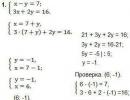
Let us give a solution to an example of a system of linear equations of class 7 using the substitution method:

As can be seen from the example, the variable x was expressed through F(X) = 7 + Y. The resulting expression, substituted into the 2nd equation of the system in place of X, helped to obtain one variable Y in the 2nd equation. Solving this example is easy and allows you to get the Y value. The last step is to check the obtained values.

It is not always possible to solve an example of a system of linear equations by substitution. The equations can be complex and expressing the variable in terms of the second unknown will be too cumbersome for further calculations. When there are more than 3 unknowns in the system, solving by substitution is also inappropriate.

Solution of an example of a system of linear inhomogeneous equations:

Solution using algebraic addition

When searching for solutions to systems using the addition method, equations are added term by term and multiplied by various numbers. The ultimate goal of mathematical operations is an equation in one variable.

Application of this method requires practice and observation. Solving a system of linear equations using the addition method when there are 3 or more variables is not easy. Algebraic addition is convenient to use when equations contain fractions and decimals.

Solution algorithm:

1. Multiply both sides of the equation by a certain number. As a result of the arithmetic operation, one of the coefficients of the variable should become equal to 1.
2. Add the resulting expression term by term and find one of the unknowns.
3. Substitute the resulting value into the 2nd equation of the system to find the remaining variable.

Method of solution by introducing a new variable

A new variable can be introduced if the system requires finding a solution for no more than two equations; the number of unknowns should also be no more than two.

The method is used to simplify one of the equations by introducing a new variable. The new equation is solved for the introduced unknown, and the resulting value is used to determine the original variable.

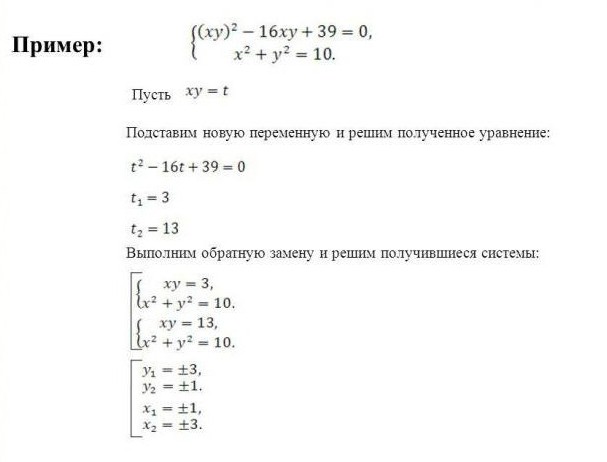
The example shows that by introducing a new variable t, it was possible to reduce the 1st equation of the system to a standard quadratic trinomial. You can solve a polynomial by finding the discriminant.

It is necessary to find the value of the discriminant using the well-known formula: D = b2 - 4*a*c, where D is the desired discriminant, b, a, c are the factors of the polynomial. In the given example, a=1, b=16, c=39, therefore D=100. If the discriminant is greater than zero, then there are two solutions: t = -b±√D / 2*a, if the discriminant is less than zero, then there is one solution: x = -b / 2*a.

The solution for the resulting systems is found by the addition method.

Visual method for solving systems

Suitable for 3 equation systems. The method consists in constructing graphs of each equation included in the system on the coordinate axis. The coordinates of the intersection points of the curves will be the general solution of the system.

The graphical method has a number of nuances. Let's look at several examples of solving systems of linear equations in a visual way.

As can be seen from the example, for each line two points were constructed, the values ​​of the variable x were chosen arbitrarily: 0 and 3. Based on the values ​​of x, the values ​​for y were found: 3 and 0. Points with coordinates (0, 3) and (3, 0) were marked on the graph and connected by a line.

The steps must be repeated for the second equation. The point of intersection of the lines is the solution of the system.

The following example requires finding a graphical solution to a system of linear equations: 0.5x-y+2=0 and 0.5x-y-1=0.

As can be seen from the example, the system has no solution, because the graphs are parallel and do not intersect along their entire length.

The systems from examples 2 and 3 are similar, but when constructed it becomes obvious that their solutions are different. It should be remembered that it is not always possible to say whether a system has a solution or not; it is always necessary to construct a graph.

The matrix and its varieties

Matrices are used to concisely write a system of linear equations. A matrix is ​​a special type of table filled with numbers. n*m has n - rows and m - columns.

A matrix is ​​square when the number of columns and rows are equal. A matrix-vector is a matrix of one column with an infinitely possible number of rows. A matrix with ones along one of the diagonals and other zero elements is called identity.

An inverse matrix is ​​a matrix when multiplied by which the original one turns into a unit matrix; such a matrix exists only for the original square one.

Rules for converting a system of equations into a matrix

In relation to systems of equations, the coefficients and free terms of the equations are written as matrix numbers; one equation is one row of the matrix.

A matrix row is said to be nonzero if at least one element of the row is not zero. Therefore, if in any of the equations the number of variables differs, then it is necessary to enter zero in place of the missing unknown.

The matrix columns must strictly correspond to the variables. This means that the coefficients of the variable x can be written only in one column, for example the first, the coefficient of the unknown y - only in the second.

When multiplying a matrix, all elements of the matrix are sequentially multiplied by a number.

Options for finding the inverse matrix

The formula for finding the inverse matrix is ​​quite simple: K -1 = 1 / |K|, where K -1 is the inverse matrix, and |K| is the determinant of the matrix. |K| must not be equal to zero, then the system has a solution.

The determinant is easily calculated for a two-by-two matrix; you just need to multiply the diagonal elements by each other. For the “three by three” option, there is a formula |K|=a 1 b 2 c 3 + a 1 b 3 c 2 + a 3 b 1 c 2 + a 2 b 3 c 1 + a 2 b 1 c 3 + a 3 b 2 c 1 . You can use the formula, or you can remember that you need to take one element from each row and each column so that the numbers of columns and rows of elements are not repeated in the work.

Solving examples of systems of linear equations using the matrix method

The matrix method of finding a solution allows you to reduce cumbersome entries when solving systems with a large number of variables and equations.

In the example, a nm are the coefficients of the equations, the matrix is ​​a vector x n are variables, and b n are free terms.

Solving systems using the Gaussian method

In higher mathematics, the Gaussian method is studied together with the Cramer method, and the process of finding solutions to systems is called the Gauss-Cramer solution method. These methods are used to find variables of systems with a large number of linear equations.

The Gauss method is very similar to solutions by substitution and algebraic addition, but is more systematic. In the school course, the solution by the Gaussian method is used for systems of 3 and 4 equations. The purpose of the method is to reduce the system to the form of an inverted trapezoid. By means of algebraic transformations and substitutions, the value of one variable is found in one of the equations of the system. The second equation is an expression with 2 unknowns, while 3 and 4 are, respectively, with 3 and 4 variables.

After bringing the system to the described form, the further solution is reduced to the sequential substitution of known variables into the equations of the system.

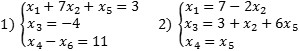
In school textbooks for grade 7, an example of a solution by the Gauss method is described as follows:

As can be seen from the example, at step (3) two equations were obtained: 3x 3 -2x 4 =11 and 3x 3 +2x 4 =7. Solving any of the equations will allow you to find out one of the variables x n.

Theorem 5, which is mentioned in the text, states that if one of the equations of the system is replaced by an equivalent one, then the resulting system will also be equivalent to the original one.

The Gaussian method is difficult for middle school students to understand, but it is one of the most interesting ways to develop the ingenuity of children enrolled in advanced learning programs in math and physics classes.

For ease of recording, calculations are usually done as follows:

The coefficients of the equations and free terms are written in the form of a matrix, where each row of the matrix corresponds to one of the equations of the system. separates the left side of the equation from the right. Roman numerals indicate the numbers of equations in the system.

First, write down the matrix to be worked with, then all the actions carried out with one of the rows. The resulting matrix is ​​written after the "arrow" sign and the necessary algebraic operations are continued until the result is achieved.

The result should be a matrix in which one of the diagonals is equal to 1, and all other coefficients are equal to zero, that is, the matrix is ​​reduced to a unit form. We must not forget to perform calculations with numbers on both sides of the equation.

This recording method is less cumbersome and allows you not to be distracted by listing numerous unknowns.

The free use of any solution method will require care and some experience. Not all methods are of an applied nature. Some methods of finding solutions are more preferable in a particular area of ​​human activity, while others exist for educational purposes.

Coursework: Determinants and systems of linear equations

1. Determinants of the second and third orders and their properties

1.1. The concept of a matrix and a second-order determinant

A rectangular table of numbers,

matrix. To indicate the matrix, use either double vertical

dashes or parentheses. For example:

1 7 9.2 1 7 9.2

28 20 18 28 20 18

6 11 2 -6 11 2

If the number of rows of a matrix coincides with the number of its columns, then the matrix is ​​called

square. The numbers that make up the matrix call it elements.

Consider a square matrix consisting of four elements:

The second-order determinant corresponding to matrix (3.1) is the number

and denoted by the symbol

So, by definition

The elements that make up the matrix of a given determinant are usually called

elements of this determinant.

The following statement is true: in order for the determinant of the second

order was equal to zero, it is necessary and sufficient that the elements of its rows (or

according to its columns) were proportional.

To prove this statement, it is enough to note that each of

proportions /

is equivalent to equality

And the last equality, by virtue of (3.2), is equivalent to the vanishing of the determinant.

1.2. System of two linear equations in two unknowns

We will show how second-order determinants are used to study and

finding solutions to a system of two linear equations with two unknowns

(coefficients ,

and free members,

are considered given). Recall that a pair of numbers

Called

solution of system (3.3), if substitution of these numbers in place

and into this system

turns both equations (3.3) into identities.

Multiplying the first equation of system (3.3) by -

And the second - on -i

then adding the resulting equalities, we get

Similarly, by multiplying equations (3.3) by - and, respectively, we obtain:

Let us introduce the following notation:

Using this notation and the expression for the second-order determinant

equations (3.4) and (3.5) can be rewritten as:

Determinant,

composed of coefficients for the unknowns of system (3.3), is usually called

determinant of this system. Note that the determinants

and are obtained from

system determinant

by replacing its first or second column with free ones

Two cases may present themselves: 1) system determinant

different from zero; 2) this determinant is equal to zero.

Let us first consider the case

0. From equations (3.7) we immediately obtain formulas for the unknowns,

called Cramer formulas:

The resulting Cramer formulas (3.8) give a solution to system (3.7) and therefore prove

uniqueness of the solution to the original system (3.3). Indeed, system (3.7)

is a consequence of system (3.3), therefore any solution to system (3.3) (in

case if it exists!) must be a solution to system (3.7). So,

so far it has been proven that if the original system (3.3) exists for

0 solution, then this solution is uniquely determined by the Cramer formulas (3.8).

It is easy to verify the existence of a solution, i.e. what about

0 two numbers and

Defined by Cramer formulas (3.8). being put in the place of the unknown in

equations (3.3), turn these equations into identities. (We provide the reader

write down the expressions for the determinants yourself

And make sure that the indicated identities are correct.)

We come to the following conclusion: if the determinant

system (3.3) is different from zero, then there exists, and, moreover, a unique solution to this

system defined by Cramer formulas (3.8).

Let us now consider the case when the determinant

system is equal zero. They can introduce themselves two subcases: Or maybe

would be one of the determinants

or , different from

zero; b) both determinants

and are equal to zero. (If

determinant and

one of two qualifiers

and are equal to zero, then

the other of these two determinants is equal to zero. In fact, let

for example = 0

Then from these proportions we get that

In subcase a) at least one of the equalities (3.7) turns out to be impossible, i.e.

system (3.7) has no solutions, and therefore the original system has no solutions

(3.3) (the consequence of which is system (3.7)).

In subcase b) the original system (3.3) has an infinite number of solutions. IN

in fact, from the equalities

0 and from the statement at the end of section. 1.1 we conclude that the second equation of the system

(3.3) is a consequence of the first and can be discarded. But one equation with

two unknowns

has infinitely many solutions (at least one of the coefficients

Or different from

zero, and the unknown associated with it can be determined from equation (3.9)

through an arbitrarily specified value of another unknown).

Thus, if the determinant

system (3.3) is equal to zero, then system (3.3) either has no solutions at all (in

case if at least one of the determinants

or different from

zero), or has an infinite number of solutions (in the case when

0). In the last

case, two equations (3.3) can be replaced by one and when solving it, one

the unknown is set arbitrarily.

Comment. In the case where free members

and are equal to zero,

linear system (3.3) is called homogeneous. Note that homogeneous

the system always has a so-called trivial solution:

0, = 0 (these two

numbers turn both homogeneous equations into identities).

If the determinant of a homogeneous system

is different from zero, then this system has only a trivial solution. If

= 0, then the homogeneous system has an infinite number of solutions(because the

for a homogeneous system the possibility of no solutions is excluded). So

way, a homogeneous system has a nontrivial solution if and only if

in the case when its determinant is equal to zero.

Systems of linear equations. Lecture 6.

Systems of linear equations.

Basic concepts.

View system

called system - linear equations with unknowns.

The numbers , , are called system coefficients.

The numbers are called free members of the system, – system variables. Matrix

called main matrix of the system, and the matrix

– extended matrix system. Matrices - columns

And correspondingly matrices of free terms and unknowns of the system. Then in matrix form the system of equations can be written as . System solution is called the values ​​of variables, upon substitution of which, all equations of the system turn into correct numerical equalities. Any solution to the system can be represented as a matrix-column. Then the matrix equality is true.

The system of equations is called joint if it has at least one solution and non-joint if there is no solution.

Solving a system of linear equations means finding out whether it is consistent and, if so, finding its general solution.

The system is called homogeneous if all its free terms are equal to zero. A homogeneous system is always consistent, since it has a solution

Kronecker–Copelli theorem.

The answer to the question of the existence of solutions to linear systems and their uniqueness allows us to obtain the following result, which can be formulated in the form of the following statements regarding a system of linear equations with unknowns

(1)

Theorem 2. System of linear equations (1) is consistent if and only if the rank of the main matrix is ​​equal to the rank of the extended matrix (.

Theorem 3. If the rank of the main matrix of a simultaneous system of linear equations is equal to the number of unknowns, then the system has a unique solution.

Theorem 4. If the rank of the main matrix of a joint system is less than the number of unknowns, then the system has an infinite number of solutions.

Rules for solving systems.

3. Find the expression of the main variables in terms of free ones and obtain the general solution of the system.

4. By giving arbitrary values ​​to free variables, all the values ​​of the main variables are obtained.

Methods for solving systems of linear equations.

Inverse matrix method.

and , i.e. the system has a unique solution. Let's write the system in matrix form

Where , , .

Let's multiply both sides of the matrix equation on the left by the matrix

Since , we obtain , from which we obtain the equality for finding the unknowns

Example 27. Solve a system of linear equations using the inverse matrix method

Solution. Let us denote by the main matrix of the system

.

Let, then we find the solution using the formula.

Let's calculate.

Since , then the system has a unique solution. Let's find all algebraic complements

, ,

, ,

, ,

, ,

Thus

.

Let's check

.

The inverse matrix was found correctly. From here, using the formula, we find the matrix of variables.

.

Comparing the values ​​of the matrices, we get the answer: .

Cramer's method.

Let a system of linear equations with unknowns be given

and , i.e. the system has a unique solution. Let us write the solution of the system in matrix form or

Let's denote

. . . . . . . . . . . . . . ,

Thus, we obtain formulas for finding the values ​​of unknowns, which are called Cramer formulas.

Example 28. Solve the following system of linear equations using the Cramer method .

Solution. Let's find the determinant of the main matrix of the system

.

Since , then the system has a unique solution.

Let's find the remaining determinants for Cramer's formulas

,

,

.

Using Cramer's formulas we find the values ​​of the variables

Gauss method.

The method consists of sequential elimination of variables.

Let a system of linear equations with unknowns be given.

The Gaussian solution process consists of two stages:

At the first stage, the extended matrix of the system is reduced, using elementary transformations, to a stepwise form

,

where , to which the system corresponds

After this the variables are considered free and are transferred to the right side in each equation.

At the second stage, the variable is expressed from the last equation, and the resulting value is substituted into the equation. From this equation

the variable is expressed. This process continues until the first equation. The result is an expression of the main variables through free variables .

Example 29. Solve the following system using the Gauss method

Solution. Let's write out the extended matrix of the system and bring it to stepwise form

.

Because greater than the number of unknowns, then the system is consistent and has an infinite number of solutions. Let's write the system for the step matrix

The determinant of the extended matrix of this system, composed of the first three columns, is not equal to zero, so we consider it to be basic. Variables

They will be basic and the variable will be free. Let’s move it in all equations to the left side

From the last equation we express

Substituting this value into the penultimate second equation, we get

where . Substituting the values ​​of the variables and into the first equation, we find . Let's write the answer in the following form

Solving systems of linear algebraic equations is one of the main problems of linear algebra. This problem has important applied significance in solving scientific and technical problems; in addition, it is auxiliary in the implementation of many algorithms in computational mathematics, mathematical physics, and processing the results of experimental research.

A system of linear algebraic equations is called a system of equations of the form: (1)

Where – unknown; - free members.

Solving a system of equations(1) call any set of numbers that, when placed in system (1) in place of the unknowns converts all equations of the system into correct numerical equalities.

The system of equations is called joint, if it has at least one solution, and non-joint, if it has no solutions.

The simultaneous system of equations is called certain, if it has one unique solution, and uncertain, if it has at least two different solutions.

The two systems of equations are called equivalent or equivalent, if they have the same set of solutions.

System (1) is called homogeneous, if the free terms are zero:

A homogeneous system is always consistent - it has a solution (perhaps not the only one).

If in system (1), then we have the system n linear equations with n unknown: where – unknown; – coefficients for unknowns, - free members.

A linear system may have a single solution, infinitely many solutions, or no solution at all.

Consider a system of two linear equations with two unknowns

If then the system has a unique solution;

if then the system has no solutions;

if then the system has an infinite number of solutions.

Example. The system has a unique solution to a pair of numbers

The system has an infinite number of solutions. For example, solutions to a given system are pairs of numbers, etc.

The system has no solutions, since the difference of two numbers cannot take two different values.

Definition. Second order determinant called an expression of the form:

The determinant is designated by the symbol D.

Numbers A 11, …, A 22 are called elements of the determinant.

Diagonal formed by elements A 11 ; A 22 are called main diagonal formed by elements A 12 ; A 21 − side

Thus, the second-order determinant is equal to the difference between the products of the elements of the main and secondary diagonals.

Note that the answer is a number.

Example. Let's calculate the determinants:

Consider a system of two linear equations with two unknowns: where X 1, X 2 – unknown; A 11 , …, A 22 – coefficients for unknowns, b 1 ,b 2 – free members.

If a system of two equations with two unknowns has a unique solution, then it can be found using second-order determinants.

Definition. A determinant made up of coefficients for unknowns is called system determinant: D= .

The columns of the determinant D contain the coefficients, respectively, for X 1 and at , X 2. Let's introduce two additional qualifier, which are obtained from the determinant of the system by replacing one of the columns with a column of free terms: D 1 = D 2 = .

Theorem 14(Kramer, for the case n=2). If the determinant D of the system is different from zero (D¹0), then the system has a unique solution, which is found using the formulas:

These formulas are called Cramer's formulas.

Example. Let's solve the system using Cramer's rule:

Solution. Let's find the numbers

Answer.

Definition. Third order determinant called an expression of the form:

Elements A 11; A 22 ; A 33 – form the main diagonal.

Numbers A 13; A 22 ; A 31 – form a side diagonal.

The entry with a plus includes: the product of elements on the main diagonal, the remaining two terms are the product of elements located at the vertices of triangles with bases parallel to the main diagonal. The minus terms are formed according to the same scheme with respect to the secondary diagonal.

Example. Let's calculate the determinants:

Consider a system of three linear equations with three unknowns: where – unknown; – coefficients for unknowns, - free members.

In the case of a unique solution, a system of 3 linear equations with three unknowns can be solved using 3rd order determinants.

The determinant of system D has the form:

Let us introduce three additional determinants:

Theorem 15(Kramer, for the case n=3). If the determinant D of the system is different from zero, then the system has a unique solution, which is found using Cramer’s formulas:

Example. Let's solve the system using Cramer's rule.

Solution. Let's find the numbers

Let's use Cramer's formulas and find the solution to the original system:

Answer.

Note that Cramer's theorem is applicable when the number of equations is equal to the number of unknowns and when the determinant of the system D is nonzero.

If the determinant of the system is equal to zero, then in this case the system can either have no solutions or have an infinite number of solutions. These cases are studied separately.

Let us note only one case. If the determinant of the system is equal to zero (D=0), and at least one of the additional determinants is different from zero, then the system has no solutions, that is, it is inconsistent.

Cramer's theorem can be generalized to the system n linear equations with n unknown: where – unknown; – coefficients for unknowns, - free members.

If the determinant of a system of linear equations with unknowns, then the only solution to the system is found using Cramer’s formulas:

An additional determinant is obtained from the determinant D if it contains a column of coefficients for the unknown x i replace with a column of free members.

Note that the determinants D, D 1 , … , D n have order n.

Gauss method for solving systems of linear equations

One of the most common methods for solving systems of linear algebraic equations is the method of sequential elimination of unknowns −Gauss method. This method is a generalization of the substitution method and consists of sequentially eliminating unknowns until one equation with one unknown remains.

The method is based on some transformations of a system of linear equations, which results in a system equivalent to the original system. The method algorithm consists of two stages.

The first stage is called straight forward Gauss method. It consists of sequentially eliminating unknowns from equations. To do this, in the first step, divide the first equation of the system by (otherwise, rearrange the equations of the system). They denote the coefficients of the resulting reduced equation, multiply it by the coefficient and subtract it from the second equation of the system, thereby eliminating it from the second equation (zeroing the coefficient).

Do the same with the remaining equations and obtain a new system, in all equations of which, starting from the second, the coefficients for , contain only zeros. Obviously, the resulting new system will be equivalent to the original system.

If the new coefficients, for , are not all equal to zero, they can be excluded in the same way from the third and subsequent equations. Continuing this operation for the following unknowns, the system is brought to the so-called triangular form:

Here the symbols indicate the numerical coefficients and free terms that have changed as a result of transformations.

From the last equation of the system, the remaining unknowns are determined in a unique way, and then by sequential substitution.

Comment. Sometimes, as a result of transformations, in any of the equations all the coefficients and the right-hand side turn to zero, that is, the equation turns into the identity 0=0. By eliminating such an equation from the system, the number of equations is reduced compared to the number of unknowns. Such a system cannot have a single solution.

If, in the process of applying the Gauss method, any equation turns into an equality of the form 0 = 1 (the coefficients for the unknowns turn to 0, and the right-hand side takes on a non-zero value), then the original system has no solution, since such an equality is false for any values unknown.

Consider a system of three linear equations with three unknowns:

Where – unknown; – coefficients for unknowns, - free members. , substituting what was found

Solution. Applying the Gaussian method to this system, we obtain

Where does the last equality fail for any values ​​of the unknowns, therefore, the system has no solution.

Answer. The system has no solutions.

Note that the previously discussed Cramer method can be used to solve only those systems in which the number of equations coincides with the number of unknowns, and the determinant of the system must be non-zero. The Gauss method is more universal and suitable for systems with any number of equations.

A system of linear equations is a union of n linear equations, each containing k variables. It is written like this:

Many, when encountering higher algebra for the first time, mistakenly believe that the number of equations must necessarily coincide with the number of variables. In school algebra this usually happens, but for higher algebra this is generally not true.

The solution to a system of equations is a sequence of numbers (k 1, k 2, ..., k n), which is the solution to each equation of the system, i.e. when substituting into this equation instead of the variables x 1, x 2, ..., x n gives the correct numerical equality.

Accordingly, solving a system of equations means finding the set of all its solutions or proving that this set is empty. Since the number of equations and the number of unknowns may not coincide, three cases are possible:

1. The system is inconsistent, i.e. the set of all solutions is empty. A rather rare case that is easily detected no matter what method is used to solve the system.
2. The system is consistent and determined, i.e. has exactly one solution. The classic version, well known since school.
3. The system is consistent and undefined, i.e. has infinitely many solutions. This is the toughest option. It is not enough to indicate that “the system has an infinite set of solutions” - it is necessary to describe how this set is structured.

A variable x i is called allowed if it is included in only one equation of the system, and with a coefficient of 1. In other words, in other equations the coefficient of the variable x i must be equal to zero.

If we select one allowed variable in each equation, we obtain a set of allowed variables for the entire system of equations. The system itself, written in this form, will also be called resolved. Generally speaking, one and the same original system can be reduced to different permitted ones, but for now we are not concerned about this. Here are examples of permitted systems:

Both systems are resolved with respect to the variables x 1 , x 3 and x 4 . However, with the same success it can be argued that the second system is resolved with respect to x 1, x 3 and x 5. It is enough to rewrite the very last equation in the form x 5 = x 4.

Now let's consider a more general case. Let us have k variables in total, of which r are allowed. Then two cases are possible:

1. The number of allowed variables r is equal to the total number of variables k: r = k. We obtain a system of k equations in which r = k allowed variables. Such a system is joint and definite, because x 1 = b 1, x 2 = b 2, ..., x k = b k;
2. The number of allowed variables r is less than the total number of variables k: r< k . Остальные (k − r ) переменных называются свободными - они могут принимать любые значения, из которых легко вычисляются разрешенные переменные.

So, in the above systems, the variables x 2, x 5, x 6 (for the first system) and x 2, x 5 (for the second) are free. The case when there are free variables is better formulated as a theorem:

Please note: this is a very important point! Depending on how you write the resulting system, the same variable can be either allowed or free. Most higher mathematics tutors recommend writing out variables in lexicographic order, i.e. ascending index. However, you are under no obligation to follow this advice.

Theorem. If in a system of n equations the variables x 1, x 2, ..., x r are allowed, and x r + 1, x r + 2, ..., x k are free, then:

1. If we set the values ​​of the free variables (x r + 1 = t r + 1, x r + 2 = t r + 2, ..., x k = t k), and then find the values ​​x 1, x 2, ..., x r, we get one of decisions.
2. If in two solutions the values ​​of free variables coincide, then the values ​​of allowed variables also coincide, i.e. solutions are equal.

What is the meaning of this theorem? To obtain all solutions to a resolved system of equations, it is enough to isolate the free variables. Then, assigning different values ​​to the free variables, we will obtain ready-made solutions. That's all - in this way you can get all the solutions of the system. There are no other solutions.

Conclusion: the resolved system of equations is always consistent. If the number of equations in a resolved system is equal to the number of variables, the system will be definite; if less, it will be indefinite.

And everything would be fine, but the question arises: how to obtain a resolved one from the original system of equations? For this there is